If you would like to try running a Python code that makes use of mpi4py on Frontera, we provide an example below. This is a program that implements a classic example in computational science: estimating the numerical value of pi via Monte Carlo sampling. Imagine you're throwing darts, and you're not very accurate. You are trying to hit a spot somewhere within a circular target, but you can't manage to do much better than throw it somewhere within the square that bounds the target, hitting any point within the square with equal probability. The red dots are those darts that manage to hit the circle, and the blue dots are those darts that don't.

Fortunately, even though you are not a very good dart thrower, you are a good random number generator, and you can put those skills to work to estimate the numerical value of pi — the ratio of the circumference of a circle to its diameter.

Exercise #1

Do a bit of math to convince yourself (assuming the darts are thrown uniformly at random throughout the square) that pi is approximately equal to 4 times the fraction of darts you have thrown that manage to land within the circle.

Exercise #2

The code below implements the key algorithmic parts — throwing random darts, figuring out which ones are in the circular target, and estimating pi from the fraction that are in the target. The code also distributes this computation using mpi4py, through a manager-worker paradigm, by having multiple processes estimate pi via this stochastic procedure: every worker throws a specified number of N darts a total of Nruns_per_worker times, and sends the results of those estimates back to the manager process to compute the mean and standard deviation of all the individual estimates. The main program estimates pi several times, for different numbers of darts N and for Nruns_total independent sampling runs, printing the mean and standard deviation of all those estimates. Fluctuations (standard deviation) in the estimates of pi should decrease approximately as 1/sqrt(N), as is typical for Monte Carlo.

Either copy and paste the code below and store it in a file named parallel_pi.py, or access the source file.

On Frontera, open up an interactive session with idev as described in the user guide. We could do something like the following to request 1 node on Frontera, in order to run our parallel code across 64 tasks:

Once we get an interactive node, we can run our code using ibrun, assuming you have loaded a python3 module:

You should see output something like:

(If you get errors involving ".cache/matplotlib/fontlist-v310.json", simply run the code again.)

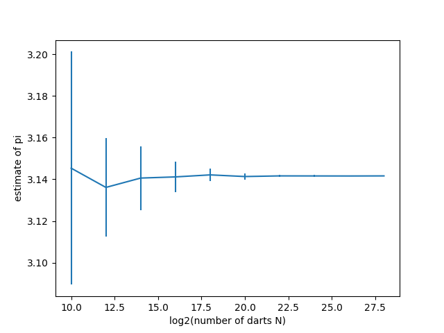
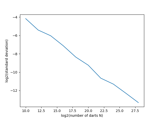
The first numerical entry on each line is the number N of random numbers sampled; the second is the mean estimate of pi; and the third is the standard deviation of all the estimates used for that N (in this example, 64 independent runs for each N). A couple figures are also produced and saved as png files in your directory (i.e., they will not be displayed on the screen) — these are shown below. The first shows convergence to an estimate of pi as a function of log2 N (i.e., log₂ N) and one showing the decrease in fluctuations in the estimate as a function of N. Specifically, since the standard deviation in the estimates should decrease as 1/sqrt(N), we can plot log2(standard deviation) vs. log2(N), and observe that the fluctuations decay on this log-log scale with slope approximately equal to -1/2. In addition, from the data that are printed out when the program is running, you should be able to observe that the fluctuations in the estimates (the last number printed out in each row) are roughly 1/2 the size of the fluctuations in the row above: because we are increasing N by a factor of 4 from row-to-row, we would expect the fluctuations to be reduced by a factor of sqrt(4)=2 on each iteration.

Plots like the above are produced as .png files when you run the provided code. To open the plots for viewing from a Frontera login node, you can try using xdg-open, assuming you are connected with ssh -X and have an X server running locally.

Exercise #3

Using some of the functions defined in the code above and some additional numpy code, make a dart plot similar to the figure at the top of the page (hint: matplotlib.pyplot.scatter). This is probably best done as a serial process, without the MPI functionality, for a relatively small number of points N.