Introduction to Parallel Computing on HPC
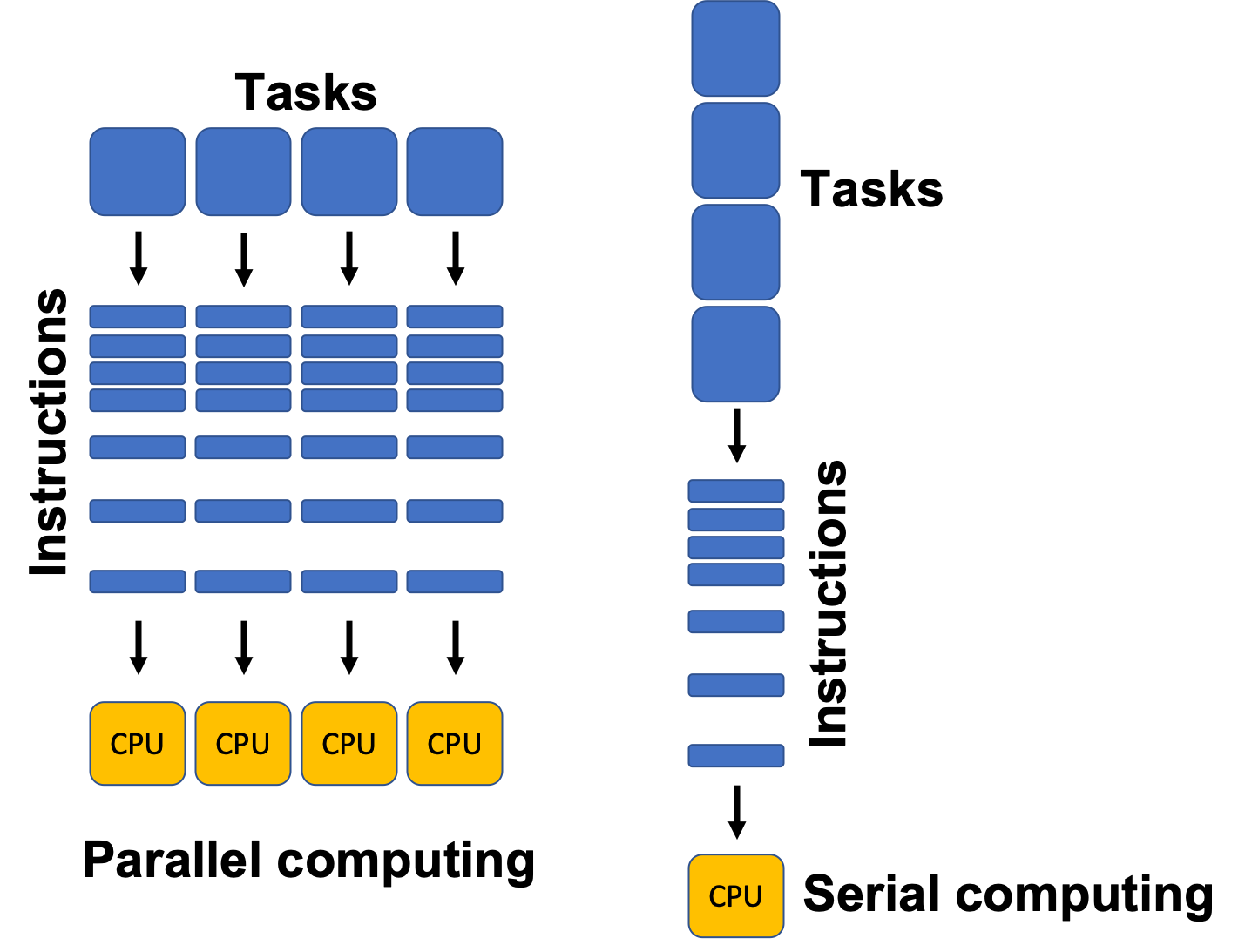
Image source: [1]
Traditionally, software has been written for serial computation where we solve a problem by executing a set of instructions sequentially on a single processor. In parallel computation, multiple computational resources are leveraged simultaneously to solve a problem and thus requires multiple processors to run. There are many problems in science and engineering that require parallel computation that runs on computational resources beyond those available on our laptops, including training neural networks. High Performance Computing (HPC) centers are a resource we can use to get access to potentially thousands of computers to execute code.
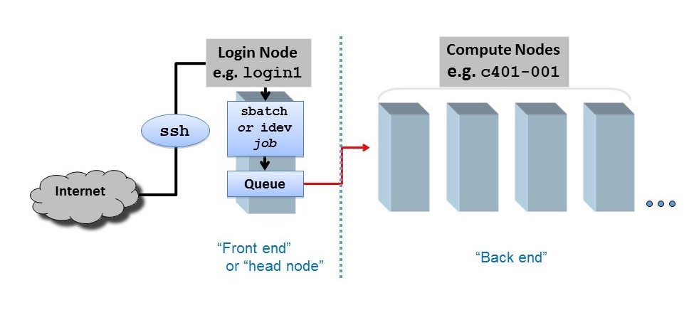
Image source: [2]
HPC centers, like the Texas Advanced Computing Center (TACC), host several supercomputers. Supercomputers, or computer clusters, are a group of interconnected computers such that they can act like a single machine. The various computers that make up the computer cluster are nodes which come in two types: login and compute. Login nodes are those that you interact with in logging on to our machines via SSH and are used for routine tasks like modifying and organizing files. Compute nodes are where the actual calculations are done and what we will utilize to parallelize the training of neural networks. There could be different types of compute nodes, for example different types of CPUs and GPUs, but we will focus on utilizing GPUs in this tutorial as PyTorch is optimized to run on GPUs. A GPU node typically consists of multiple GPUs. Each GPU on a node is identified with a unique integer referred to as local rank (See Figure 4).
Image source: [3]
PyTorch has tools for checking the number and types of GPUs available. For example, you can check if GPUs are available with is_available(). You can determine the number of GPUs you have available via device_count(). You can also determine the local rank of the device you are currently using with current_device(). The following lab will demonstrate these tools.
In this notebook, we will introduce how to parallelize the training process of a CNN classifier across multiple GPUs on a single node. One of the main challenges of parallelizing code is that there is often a need for the various processes to communicate with one another. Let’s say for example I want to solve the following set of equations:
One way to parallelize solving this simple set of equations is to use two processors to compute \(A\) and \(D\). There are a few things that need to happen after \(A\) and \(D\) are computed on the 2 processors:
- Synchronization: Both processes wait until all members of the group have reached the synchronization point. Both \(A\) and \(D\) need to both have been computed to move on to computing \(G\). Synchronization can be a time bottleneck in parallel computing.
- Data Movement - Once \(A\) and \(D\) have been computed, the values of \(A\) and \(D\) need to reside on the same processor. This is where data movement comes in (see Figure 5 for examples of different types of data movement).
- Collective Computation - In this example, one processor collects data (values of \(A\) and \(D\)) and performs an operation (min, max, add, multiply, etc.) on that data.
Image source: [4]
All 3 of these steps typically need to be programmed when building parallelized code and can often be time bottlenecks.
Now that we have introduced a little bit about parallel computation, HPC terminology and how communication works, let’s look at one algorithm that is used to parallelize the training of neural networks, Distributed Data Parallel (DDP).
CVW material development is supported by NSF OAC awards 1854828, 2321040, 2323116 (UT Austin) and 2005506 (Indiana University)