This exercise is inspired by the Demonstration provided by Killian Weinberger of the Cornell University Department of Computer Science in this video from a 2021 Quantum Matter Summer School. The demo is a small part of a much larger video, and the link above goes to that chapter of the video. But you might want to back up a chapter or two to see Killian's explanation of what the demo is doing. Or you might want to watch the entire thing, since it's very interesting and informative!

As noted in the preceding introductory material, neural networks are basically learning to map inputs to outputs. They are function approximators. And this demo that Killian Weinberger and Paul Ginsparg constructed does a nice job of demonstrating that learning process, in the relatively simple example of a regression to a set of data points in two dimensions. Their demo is much more compelling than the exercise included below — in its use of interactive graphics, real-time model updating, and auxiliary graphics that demonstrate the structure and status of the neural network. But the exercise below is at least a start in creating something along those lines, and perhaps a substrate for you to work with if you aspire to building something like what is shown in the video.

There are a few points worth making about how this exercise differs from the one shown in the video:

• This exercise uses TensorFlow and Keras to build a neural network, whereas it appears that the demo in the video encodes the network and its action directly using the numpy library. The architecture of the TensorFlow/Keras network model, however, is intended to mimic that displayed in the video.
• This exercise generates a set of points to fit programmatically, rather than allowing the user to click in a plot window and have the points appear.
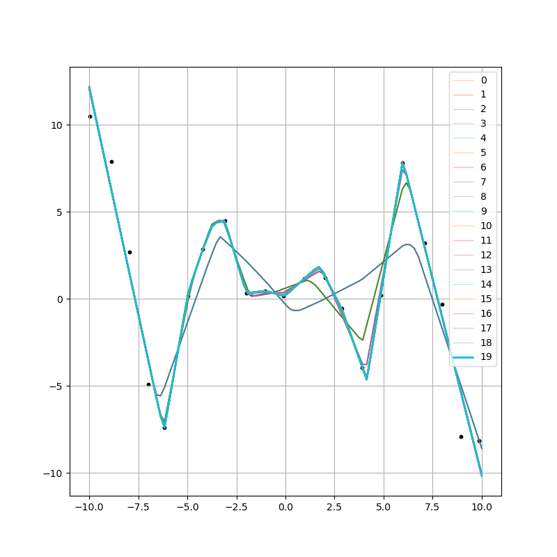
• Because this exercise does not generate animated graphics like in the video, it instead does a sequence of fits, and plots the current fit at regular intervals in the training process. Therefore, there are multiple fitting curves drawn, which presumably improve in their approximation of the data as the fitting progresses, and converge to a best fit during the later stages.
• You can download and run the exercise code below, assuming you have the proper software environment configured, which in addition to tensorflow would also require matplotlib for plotting. It's good to run it multiple times, since both the points generated differ randomly from run to run, as do the initial parameters assigned to the edges and nodes of the network. If you run it multiple times, you can see that sometimes it does a good job of fitting the data, and sometimes it does not. (An example of such of fit is shown in the figure below. The demo in the video always seems to do a good job, given a sufficient number of nodes in the hidden layer.) You could experiment with different aspects of the fitting code to see if different choices of optimization algorithms makes a difference in the outcome.

So feel free to download and run the code below, and consider some of the points raised above. You can modify the code to provide a different number of data points, or to use a different number of nodes in the hidden layer, or whatever. Enjoy!