To complement its two-dimensional line plots, MATLAB also provides the surf function for making three-dimensional (surface) plots. Plots of this sort are useful in many areas of science and engineering, in particular for making diagrams and teaching simple concepts in optimization and vector calculus. Unfortunately, creating surface plots requires the helper function meshgrid in order to work correctly.

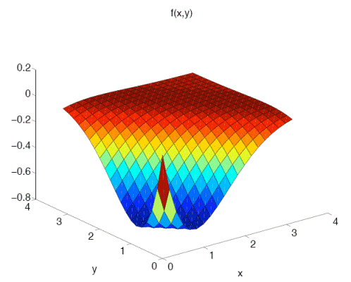
Below we create a function f(x,y) composed of sinusoids and exponentials, which also happens to be symmetric in x and y, to illustrate the process of creating a surface plot in MATLAB. We plot this smooth example function on the square domain [0,pi]^2, using N1 points in the x-direction and N2 points in y. In this particular case, N1=N2=20 but in general they need not match. After creating the one-dimensional arrays x_array and y_array, we then proceed to loop over them with nested for loops, and fill in the values of the smooth function we plan to plot.

N1 = 20;
N2 = 20;
x_array = linspace(0, pi, N1);
y_array = linspace(0, pi, N2);

for n=1:N1
    for m=1:N2
        x = x_array(n);
        y = y_array(m);
        f(n,m) = -2*exp(-x)*exp(-y)* ...
                (sin(y)*cos(x) + cos(y)*sin(x));
    end
end

Since some forms of the surf command take three matrix arguments as input, we must perform an intermediate processing step on x_array and y_array before passing them to the surf functionline 3. This intermediate processing step is handled by the meshgrid command line 2, which takes two vectors as input and returns two matrices in the format required by surf. The surf format is essentially a matrix X with the x_array values repeated row-wise and a matrix Y with the y_array values repeated column-wise.

clf('reset'); % delete graphics objects from prior example
[X,Y] = meshgrid(x_array,y_array);
surf(X,Y,f');
view(3);
xh=xlabel('x');
yh=ylabel('y');
th=title('f(x,y)');
print('MySurfacePlot','-dpdf');

We call the surf command and pass f' (the transpose of f) instead of f, since by default the surf function plots ordered pairs (x(j), y(i), f(i,j)) rather than (x(i), y(j), f(i,j)). Finally, in addition to some simple labels, we also set the default three-dimensional view by calling view(3). Note that the view command can also be used to set the azimuthal (AZ) and elevation (EL) angles directly, but the default three-dimensional view, AZ=-37.5, EL=30 is sufficient for this example. The resulting three-dimensional plot, when printed as a PDF, is sharp-looking and scales well for presentation on any size document or display device. Note, we used clf('reset') to prevent prior graphics objects from showing up in our figure, but you might not want to reset the objects if you are making a composite figure.