Structured data abound in data science and other scientific disciplines, especially in the form of regular data well represented by homogeneous arrays, and tabular data which can hold different types of data in each column. Two fundamental packages for dealing with these are NumPy and Pandas. We introduce here the key objects and data structures provided in these packages, which will be fleshed out in greater detail throughout this tutorial.

Arrays in NumPy

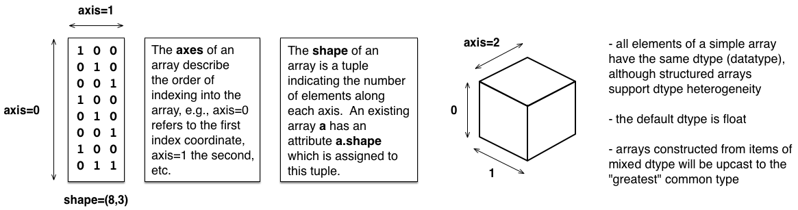
Support for multidimensional array data has long been provided by NumPy, the workhorse and cornerstone of the Python ecosystem for scientific computing. Here we will briefly introduce NumPy arrays, which share some features with Python lists, in that they support indexing and slicing by position in an array or list (albeit in higher dimensions for multidimensional arrays). Whereas lists can hold objects of different types, a given NumPy array is homogeneous in type (defined by its so-called dtype). Understanding the anatomy of a multidimensional array — in particular the shape and axes of an array, as depicted in the figure below — is useful in working with these datatypes, as well as with Pandas dataframes, as described below. Arrays are efficient computational structures, in large part because they can be operated on at a high-level, using array-level operations, rather than having to explicitly loop over their elements and act on them one at a time in Python. This functionality is described in more detail in our companion material on NumPy, as well as its role in supporting Python for High Performance.

Anatomy of an Array

Indexing and slicing of arrays

Arrays are indexed and sliced by positional indices, enclosed in square brackets, extending the notions supported by Python lists to multiple dimensions. Positional indices are zero-offset, i.e., the first element of an array is at position 0. Many variants of array indexing and slicing are described in the NumPy documentation, including both Basic and Advanced indexing. The following code snippets show just a few examples of the sort of indexing and slicing available with NumPy arrays.

import numpy as np
x = np.random.random((3,4,5))   # x is a uniform random 3D array with shape=(3,4,5)
x[0,1,2]  # extract element from x at position (0,1,2)
x[0]      # extract row (axis=0) at position 0, yields 2D array of shape (4,5)
x[:,2]    # extract column (axis=1) at position 2, yields 2D array of shape (3,5)
x[0:2,1:3,3:5]  # extract 2x2x2 subarray with specified slices along each index

DataFrames and Series in Pandas

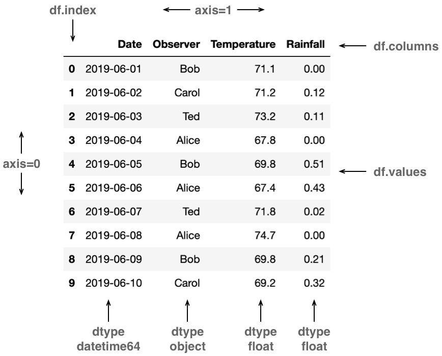
Pandas is a central Python library for data science, especially useful for dealing with tabular data of the sort that one might find in a spreadsheet or a csv-formatted file. Because of its broad applicability, much of the material presented in this tutorial uses Pandas and its associated data structures. Pandas builds on many of the important concepts introduced with NumPy (and in fact uses NumPy under the covers for many of its operations), and defines two important new classes of objects: DataFrames and Series, which link together table data with identifying information such as row and column names. Series are similar to one-dimensional NumPy arrays, with a single dtype, although with an additional index (list of row labels). DataFrames are an ordered sequence of Series, sharing the same index, with labeled columns. This is depicted in the figure below, showing various attributes of a dataframe (df), and noting the use of NumPy concepts such as axis and dtype. Each column of the dataframe, if sliced out on its own, corresponds to a Series with its associated dtype.

Anatomy of a DataFrame

Indexing and slicing of DataFrames and Series

Indexing and slicing of Pandas DataFrames and Series, while similar in spirit to NumPy, are different in several details, as discussed below. Online documentation provides more information about Pandas indexing.

• There are multiple mechanisms for indexing or slicing out content from a DataFrame or Series: [ ], loc and iloc. For [ ] and loc, indexing and slicing are based on labels (i.e., index and column labels). For iloc, indexing and slicing are based on position.
• Bracket-based indexing is column-based for DataFrames and row-based for Series. For a dataframe df, df[colname] selects the column with name colname. Multiple columns can be selected with a list of column names, e.g., df[[colname1, colname2]].
• Indexing using loc enables access via both row and column labels, using a similar notation as in NumPy. For a dataframe df, df.loc[rowname, colname] selects the item in row rowname and column colname. df.loc[rowname] selects all columns in row rowname, and is equivalent to df.loc[rowname, :]
• Slicing by either row or column labels using loc is inclusive at both the start and stop labels (unlike in NumPy, where slicing stops one position short of the stop argument), and respects the order of row and column labels in the index and columns, respectively. For a dataframe df with columns ['a', 'b', 'c', 'd', 'e'], then df.loc[:, 'a':'c'] will return the subframe consisting of all rows and the columns 'a', 'b', 'c'.
• Slicing by either row or column positions using iloc is inclusive at the start but exclusive at the stop position (as in NumPy, and for Python lists).