Now that we've learned about basic scaling behaviors, let's try to estimate how a particular code (yours!) might perform on different numbers of PEs. The model that we construct for making such an estimate will help us see where the code's scalability can be improved. To accomplish our goal, we will need to add the one ingredient that's been missing from our discussion so far: parallel overhead. We'll be focusing on communication time, since it's somewhat easier to account for that part, while neglecting another important source of parallel overhead, synchronization time.

A simple model of how some parallel applications work is that the program does many iterations where there is a fixed amount of computational work for each iteration, then the program stops doing floating point calculations in order to send and receive messages (Larry P. Davis et al., 2007). We assume that for each worker, the time to send messages is split between time to initiate the messages to the other workers, and time to send the bulk of the data contained in the messages:

\[total~time = computation + message~initiation + message~bulk\]

Let's consider the parallel speedup of a fixed workload due to N workers, which means we're looking at strong scaling, although we could certainly construct a similar performance model to handle weak scaling. For each worker, the basic computational cost can be estimated in a manner similar to Amdahl's Law, which accounts for the non-parallelizable portion of the work:

\[computation = {workload \over N} + serial~time\]

But we also want our model to include parallel overhead due to message passing, which is ignored by Amdahl's Law. We compute the message costs as follows:

\[message~initiation = (number~of~messages) \times latency\] \[message~bulk = {(size~of~all~messages) \over bandwidth}\]

We need to remember that the number and size of messages might themselves depend on N. We therefore assume a model of the form:

\[total~time = {workload \over N} + serial~time + (k_0 \times N^a) \times latency + {(k_1 \times N^b) \over bandwidth}\]

In practice, the way to discover the effective dependence of speedup on N is by fitting a formula like the one above to benchmark data. Often you'll find that the mere presence of serial time (Amdahl's Law) isn't the dominant contribution to slowing your benchmarks. First of all, communication time can resemble serial time, if a and b in the above formula turn out to be close to zero. This situation can actually occur in cases where (1) the message count and size per worker are fixed, and (2) all communication is done in parallel over a dense network like Frontera's. But worse, as a problem is split into smaller pieces, the tasks may need to send more messages with a greater total number of bytes.

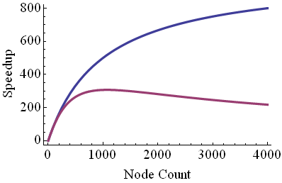
Here are a pair of speedup curves based on our simple performance model. In the standard speedup calculation, the right hand side of the equation with a and b comprises the denominator: the shape of the blue and purple curves comes from the four terms in it. For small numbers of tasks, the first term is largest, yielding linear speedup. The speedup begins to bend away from linear due to the serial time, plus any communication time that is independent of N. For the purple curve, though, one or both of the terms at the end becomes dominant, and the curve flattens much more quickly. Beyond some large number of tasks, the communication overhead may even cause the total time of the computation to increase with N, rather than decrease. Thus the speedup becomes a slowdown.