Nearly all modern processors are equipped with certain extra-wide registers that are designed to hold multiple operands, together with specialized functional units that are able to execute the identical instruction on all data items simultaneously. If these vector processors can be utilized successfully, it means that multiple flops will occur in a single cycle for a big performance boost. Getting one's code to take advantage of this special hardware is known as vectorization. No code optimization can be considered complete without it.

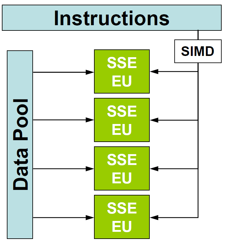
The main object of vectorization is to arrange one's code, especially the inner loops, so that the compiler is able to use SIMD (Single Instruction, Multiple Data) constructs to carry out the loop computations. Given vectorizable inner loops with independent iterations, most compilers will generate code that employs Intel's Streaming SIMD Extensions, or SSE, assuming the hardware target is an Intel (or compatible) processor. Many compliers can also make use of the Advanced Vector Extensions or AVX instruction set for the latest generations of Intel hardware. These SIMD instructions operate on multiple arguments simultaneously, as if they were in parallel Execution Units (EUs, shown below).

What makes a loop vectorizable? Generally, the loop body should consist of a series of independent, elementwise operations involving one or more arrays (vectors). In that case, the compiler can apply SIMD instructions to segments of the array(s). Such instructions will work on the elements in groups of 8 or 16 (say) rather than individually. A simple sum of two vectors provides an easy example of a vectorizable loop in C:

More complex types of array operations can be vectorized by the compiler as well. The following matrix-vector product turns out to be vectorizable:

The above example isn't so trivial. As written, the value stored in b[i] by the code at iteration j depends on the result from the previous iteration j-1. However, the compiler is smart enough to unroll the inner loop and create several independent partial sums, which are combined into a single result for b[i] at the end of the inner loop. Thus the final, compiled code may run many times faster than it would otherwise. Clearly the compiler is your friend!

Once your code becomes too complex, though, the compiler can be hindered. Let's say the above loops are placed into a function. The compiler may then decline to vectorize anything, because it has no guarantee that b, a, and x point to separate, non-overlapping areas of memory. Likewise, if any sort of branch or switch is inserted into the computation, the compiler is prevented from vectorizing the loop, because it is no longer safe to assume that exactly the same operations apply to all the elements:

But sometimes it is possible to make use of the many standard math operations that are vectorized for you. Thus the following rewrite of the above loop should vectorize successfully:

If you'd like to learn more about what works and what doesn't when writing auto-vectorizing code, you can check out the Virtual Workshop's Vectorization roadmap.

The vector registers that execute the SSE and AVX instructions are fixed in width, so the number of operations that can be executed simultaneously depends on the number of bytes in the operands. Going as far back as Intel Sandy Bridge, the AVX vector registers were 256 bits (32 bytes) wide, so an AVX operation could be performed on either 8 floats or 4 doubles, all in parallel, during a single cycle.

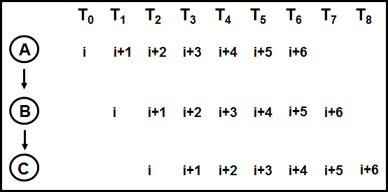
Another form of built-in "micro-parallelism" that can take place within a single processor core is pipelining. If a computation consists of several independent stages, and if multiple operands can be processed one after the other, then it may be possible for these operands to proceed through the successive stages in assembly-line fashion. Each operand advances by one stage simultaneously and in parallel during every cycle. This situation typically occurs in a load-operate-store sequence: the next operand is always being loaded while the newest result is being computed, and while the result of last cycle's operation is being stored.

In the above figure, we see how a pipeline greatly increases throughput. In this illustration, all 7 data items (indexes i to i+6) have all been processed at the end of 9 time intervals (T_0 to T_8), whereas if no pipeline existed the same processing would take 21 time intervals (7 times 3). The speedup is less than a factor of 3 because it takes a couple of steps to fill the pipeline to start with. The cost of filling the pipeline becomes relatively unimportant when there are many items to be processed.

Another common pipelining scenario is the FMA or fused multiply-add, which is a fundamental part of the instruction set for some processors. The basic load-operate-store sequence simply lengthens by one step to become load-multiply-add-store. The FMA is possible only if the hardware supports it, which is true for nearly all modern processors.