Dimensionality reduction is another set of techniques in unsupervised learning where approximate representations of datasets are developed involving fewer independent degrees-of-freedom (so that the dimensionality of the dataset is reduced in the approximation). Broadly speaking, dimensionality reduction methods appear in many different situations and in conjunction with many different methods. If one has time-series data, for example, one might choose to compute a Fourier transform of the data to convert it to the frequency domain: often one just wants to work with that full complement of frequency data, but sometimes one can pull out a few dominant frequency modes that capture most of the variation in the original signal, and those few modes can be used to develop an approximate representation of the signal that is much smaller and of lower dimension.

Various dimensionality reduction methods have been developed to support these sorts of data reductions and approximate representations. Whether or not there is an effective low-dimensional representation depends on the data, but it is often the case that "big data are not as big as they seem", in that datasets embedded in some high-dimensional data space actually lie along or within some lower-dimensional manifold contained in that space. Thus dimensionality reduction often has contained within it in a process of "manifold learning", that is, inferring (learning) what low-dimensional manifold describes the geometry of a dataset.

The most widely used dimensionality reduction method is probably Principal Components Analysis (PCA). At its root, PCA attempts to model a cloud of data points in some data space as an ellipsoid, and to identify the principal axes of that ellipsoid as the source of a low-dimensional description. These principal axes are the (orthogonal) directions of maximum variation in the dataset: the first principal component corresponds to the longest dimension of the data cloud, etc. PCA works well if your data is in the shape of an ellipsoidal cloud, but works less well if it has some other shape, even if that shape involves locally a lower-dimensional structure, such as the classic "swiss roll" structure (a 2D manifold embedded in 3D), or a piece of spaghetti twirled up on itself (a 1D manifold embedded in 3D). Nonlinear dimensionality reduction methods aim to extract these sorts of manifolds, and we will consider one such method here: T-distributed Stochastic Neighbor Embedding, or TSNE (pronounced "tee-snee").

TSNE is often used to reduce a dataset from some large number of dimensions down to a few dimensions (usually 2, sometimes 3) to allow for data visualization. Like many nonlinear methods, it aims to preserve local structure in a dataset by placing similar data points nearby each other (as "neighbors"), even if any projection from many dimensions down to 2 will invariably involve some distortion (such as we see in 2D maps of the surface of the earth). TSNE is supported by scikit-learn, and documented online. We will use this method to visualize the batting data we considered above in the context of clustering (pl_bat_per_ab), in order to generate a global map of the batting characteristics of every MLB player. We will visualize that map using the interactive Bokeh tools we have examined previously in order to provide a platform for users to explore that map in detail. The associated Jupyter notebook will enable you to run this code on your own, although you will be able to interactively explore the map below without having to run the code yourself.

In the code cell below, we import the TNSE object from sklearn.manifold, which provides a variety of methods for manifold learning. Then we write a small function to take an array of numerical data representing a set of feature vectors (in this case, the scaled batting data we constructed previously when doing clustering, Xsc) as well as a set of labels for those data, which in our case will be the playerID that is associated with each feature vector. We then run the TSNE analysis (this might take a few minutes to complete), and then clean up the resulting dataframe (which we call dfe, short for "dataframe embedding").

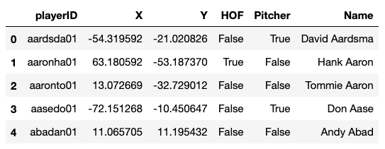
Because we'll want to visualize the data alongside some other information, let's augment our new dataframe dfe. Specifically, let's add a few columns describing whether or not a player is in the Hall of Fame (HOF), whether or not they were a Pitcher, and their name to make their identity more obvious. We'll take a peek at the dataframe once we're done.

The embedding produces (X,Y) coordinates for each player. Because TSNE is stochastic, the actual layout and appearance in this 2D space will change from run to run, but local structures and relationships ought to be robust across runs.

In order to visualize this dataset, we can leverage the interactive plotting functionality supported by Bokeh, which we introduced earlier in this tutorial in the context of Twitter data.

By rendering different parts of the augmented dataframe in various ways, we can produce a map that fleshes out the picture above, providing insights into the differences between pitchers and position players, and between HOF inductees and those not in the HOF. Bokeh produces an HTML file with all this information embedded, and by panning, zooming, and hovering over data points to see additional statistics, one can explore this map of hitting in baseball. Below the following code cell is a static image of the rendering of the map, but that image is just a hyperlink to the separate HTML page that will open if you click on the image link. So click on the image at the bottom of the page and explore the world of hitting in baseball.