Sometimes we have a model that we'd like to fit to associated data. Fitting model parameters to data is known as parameter estimation. In some cases, we might have a statistical model with an assumed functional form between model inputs and outputs, such as the case of linear regression that we examined previously. In other cases, we might have a mechanistic or process-based model, where the functional relationship between inputs and outputs is not explicitly stated, but is an emergent outcome of the action of the model. For the sake of simplicity, we will not consider the latter case here, but some of the techniques presented here are certainly applicable to that situation. Because the process of optimization is abstracted by the SciPy package, we can estimate model parameters (i.e., determine the set of parameters that optimally fits the data) regardless of whether the function that maps parameters to model outputs has an explicit functional form or is the implicit result of a mechanistic model (such as a set of differential equations that can be integrated and whose outputs are dependent on parameters). In this tutorial, we'll consider a simpler model of some of the baseball data, derived from the rich history of data analytics in baseball — please follow along in the associated Jupyter notebook if you would like to run the code yourself.

Baseball has long been a game of numbers and statistics, leading to the development over the past few decades of a number of novel and advanced statistical characterizations of individual and team performance, as well as a culture of sports analytics driving decision-making by professional teams and fan-engagement by those who follow the game. "Sabermetrics" is a branch of advanced statistical modeling for baseball, named after the Society for American Baseball Research (SABR). The term was coined by Bill James, widely regarded as the founder of modern baseball analytics.

One novel statistic that James invented is the "Pythagorean winning percentage" or "Pythagorean expectation", which led him to formulate what is sometimes referred to as the "Pythagorean theorem of baseball". This statistic essentially encapsulates a model that aims to predict how many games a baseball team will win just based on the number of runs they score and the number of runs they allow. In order to win a game, a team must score more runs than it allows, but how those quantities pile up over the course of many games was the subject of James' inquiry. The model aims to predict a team's expected win ratio (wins W / total games played G) based on the number of runs it scores (R) and the number of runs it allows (RA). As formulated by James,

\[W/G = \frac{R^2}{R^2 + RA^2} = \frac{1}{1+(RA/R)^2} \]

The fact the formula involves a sum of squares is suggestive of the theorem describing the relationship among the lengths of the sides of a right triangle, formulated by Pythagoras (and hence the name). In subsequent work, the value of the exponent 2 has been allowed to vary, to determine better fits to the data, as we shall examine below.

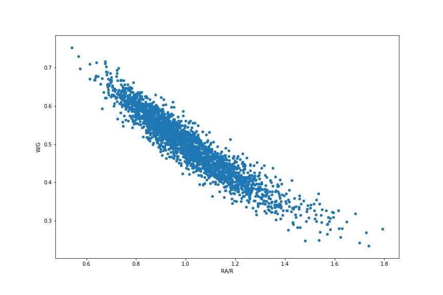
We can examine this relationship in the data by augmenting the teams dataframe with some additional columns. We'll start by filtering the teams dataframe only going back to the year 1900, which is the beginning of baseball's "modern" era — we'll call this dataframe teams00. In the dataframe, the columns 'W', 'G', 'R', and 'RA' refer to wins, games played, runs scored, and runs allowed, respectively. Then we can augment the dataframe with additional information about win ratio ('W/G') and run ratio ('RA/R'). Let's make a scatter plot of W/G vs RA/R:

As noted, even though the data relationship was originally formulated with an exponent of 2, we can generalize the model to allow for any exponent, which we represent here as \(\mu\):

\[W/G = \frac{R^\mu}{R^\mu + RA^\mu} = \frac{1}{1+(RA/R)^\mu} \]

In doing so, we can fit this generalized model of the data to identify the value of the exponent that best fits the data. The SciPy package, and in particular, the module scipy.optimize, provides a number of functions for carrying out these sorts of optimizations and data fits. We will use the function curve_fit to extract the best-fitting value of the Pythagorean exponent, by first defining a function (named pythag) that we want to optimize, and then passing that function along with the data to curve_fit.

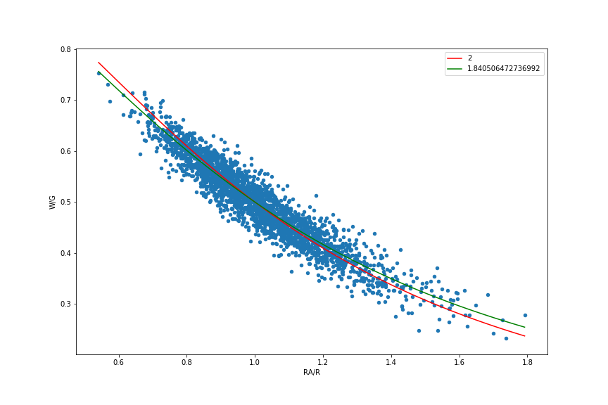
When we carry out this curve fit, we find an optimal exponent \(\mu\) of approximately 1.84, rather than 2 as originally suggested by James. Below is a replotting of the data, along with both the optimal fit to the data computed above, and the original model with the exponent equal to 2. The value of 1.83 is conventionally reported by BaseballReference.com as an optimal fit, but their estimation process is not obviously documented. In addition to tweaking the exponent to find the best fit of a "pythagorean-type" model to the data, several writers have introduced other model variants to get better predictors of a team's performance.

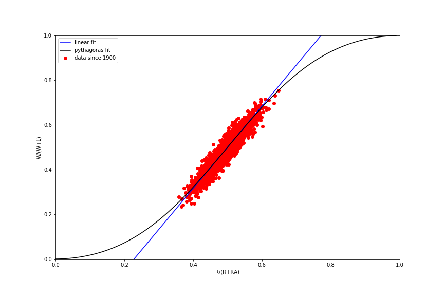
If this all seems a little opaque, part of the reason the Pythagorean formulas have the nonlinear forms they do is that the ratio of runs allowed to runs scored (RA/R) is not really the best variable for characterizing these relationships. Ben Vollmayr-Lee has an excellent post that demystifies these various models and provides a systematic way of thinking about the relationship among different model variants. By changing variables as Vollmayr-Lee suggests and reproducing (more or less) one of his plots, we can see that the data basically represent a linear relationship between fraction of games won (W/(W+L)) and fraction of runs scored (R/(R+RA)), centered about the point (1/2, 1/2). A nonlinear pythagorean model basically helps to fit the tails of the dataset a little better to address the fact there are diminishing returns in the data: after some point, scoring lots of runs (or giving up lots of runs) has less impact on the overall win ratio. See Vollmayr-Lee's post for details.

As noted in the introduction, these same sorts of parameter estimations can be carried out using more complex mechanistic models. If we had a model that consisted of a set of coupled differential equations that we need to integrate, we could define a function analogous to pythag that depends on model parameters, and then pass that function to curve_fit or some other optimization routine to determine what parameters best fit the outputs of the model to the data we want to analyze. This sort of parameter estimation is widespread in many fields, including systems biology, although this process is not without its own complexities.