Statistical modeling of data has a rich history and is widely supported by a number of different packages and computational environments. These environments typically provide support for a variety of activities, including but not limited to: regression, model fitting, parameter estimation, and hypothesis testing. Within the Python Data Science Ecosystem, much of this functionality is provided by both the Statsmodels and SciPy packages. We'll consider Statsmodels first here, and then examine SciPy later in the context of integrating data and models.

Linear Regression

Statsmodels is a package that provides support for the estimation of many different statistical models, conducting statistical tests, and carrying out statistical data exploration. It provides functionality similar to that offered by other widely used statistical modeling environments, such as R, SAS, and Minitab. Among other things, it provides a number of classes and functions for building linear regression models, generalized linear models, time series analysis, and state space models. In this tutorial, we will just consider the simplest such application, namely Ordinary Least Squares (OLS) linear regression. We will do so using the data from the Baseball Databank -- you can follow along in the associated Jupyter notebook if you're interested in carrying out these analyses on your own.

Let's start by filtering our batting dataset a bit to consider only those statistics starting in the year 1900, which is the beginning of baseball's "modern" era. Because the rules of the game changed a lot in the early years of baseball, and were mostly codified starting in 1900, this is a useful way to remove some of the systematic variation associated with those changes. We saw in previously that the history of hitting in baseball changed considerably after those early years.

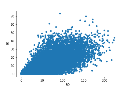
We'll filter by date to capture the modern era, and drop any missing data since that will interfere with the statistical analyses that follow. We'll call this new dataframe batting00, and then we will augment the dataset as we did previously in order to identify the number of one-base hits ('1B', or singles) that each player had. Then we'll make a scatterplot of the relationship between home runs (HR) and strikeouts (SO).

Linear regression assumes a linear relationship between a dependent variable and one or more independent variables (which statsmodels refers to as endogenous and exogenous variables, respectively). Let's perform linear regression between the strikeout and home run data plotted above.

We do this using the statsmodels.api module, which is conventionally imported as sm. We begin by importing the module and defining the endogenous (y) and exogenous (X) data we want to use for the regression. By default, statsmodels does not estimate a y-intercept for a linear regression, but we can trigger such an estimation by adding a constant term to the model; this has the effect of adding a column of ones to the X data:

Having defined the data of interest, we can construct a model of the class sm.OLS, for Ordinary Least Squares, and we can fit the model to the data. The results of the fit can then be printed out.

Many statistics are represented here, and readers are directed to the OLS documentation for details. Of primary interest are the estimated parameters for the linear fit, along with their statistical significance. Those are presented in the middle panel of the table above, describing the values of the coefficients (coef) for both the constant term, i.e., the y-intercept (constant), and the slope relating SO to HR. To assess significance, statsmodels carries out a t-test to determine if the estimated coefficients are statistically different from zero. The column P>|t| indicates the results of these tests. In both case, the probability that the coefficient could have its stated values in a statistical null model with zero mean and unit variance is 0.000 (out to 3 decimal places), indicating statistically significant estimates.

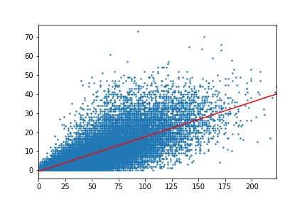
Statsmodels provides capabilities for plotting the results of the regression analysis (in this case, a straight line), contained in the sm.graphics module. Since statsmodules uses matplotlib for its graphics, we can tweak the statsmodels plot using additional matplotlib commands in order to plot the regression results alongside the original data.

Above, we carried out a simple univariate regression to identify how HRs are related to SOs. Of course, multivariate regressions are also possible, to identify how an endogenous variable depends upon multiple endogenous variables. Statsmodels supports these kinds of analyses; the basic code is shown below, with results of such an analysis contained in the accompanying notebook.