Descriptive statistics involves generating statistical summaries of data, without necessarily developing mathematical models of those data. As discussed, NumPy arrays and Pandas dataframes and series support a wide variety of aggregate operations. Many of these operations generate descriptive statistics that are useful for summarizing the character of datasets. We will investigate a few of these operations here.

We'll consider here a few examples using pandas in conjunction with some of the Baseball Databank data. Feel free to follow along in the accompanying Jupyter notebook to step through all the details.

The teams dataframe in the Baseball Databank contains information about the performance of each team during a given year over the history of major league baseball. Since the number of games played by each team during a season has changed over time, it is useful to augment the dataframe with a few more columns to normalize with respect to that variation in games played. We'll add two more columns, named RperG (runs per game) and WperG (wins per game), to get the average number of runs and wins per game, respectively. (In principle, this could be done for every entry in the teams dataframe, but we will only consider these two statistics here.)

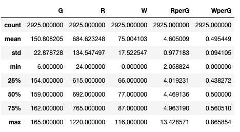
As noted, pandas provides numerous functions and methods for calculating various statistical summaries of a dataset. Several of these are conveniently bundled up in a meta-summary, supported by the describe method on a dataframe. This method computes means, standard deviations, minimum values, maximum values, and 25%/50%/75% quartile levels across all numerical columns in a dataframe, providing a quick summary of the data. Note that the object returned by the describe method is itself a dataframe, with the summary names serving as the dataframe index (row labels).

There are so many columns in this dataframe that we would need to scroll to the right within the notebook to see them all. We can restrict our focus to just a few of them if we want, by identifying just a subset of the columns for summary, such as:

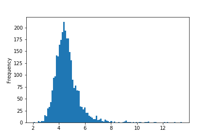
We see that the runs per game (RperG) has a mean of approximately 4.61 and a standard deviation of approximately 0.98. We can visualize this by plotting a histogram of the RperG data, using the command: teams['RperG'].plot.hist(bins=100).

By default, the summary statistics computed are for all the data in the dataframe. Sometimes it is useful to break up the data into subsets before computing data summaries. We previously introduced groupby operations to split a dataframe into subsets before applying an aggregation function to each group. We previously considered the situation where we grouped data according to a shared categorical label (such as a playerID, for the case of baseball players). But pandas also provides very useful tools for splitting a dataset into groups by binning of numerical data, similar to how data are grouped into bins when one plots a histogram, as above.

The pandas function pd.cut cuts a dataframe or series by grouping a particular column into equally spaced bins, as is done with a histogram. The function pd.qcut cuts a dataframe or series into bins of variable size such that each bin contains (approximately) the same number of entries. The qcut function takes a parameter q that indicates how many bins to cut into, so q=4 would split the data into quartiles, q=5 into quintiles, etc.

Strictly speaking, what cut and qcut both do is introduce a new data label for each row indicating the numerical interval described by a bin. In other words, it converts numerical values into categorical values, the latter being the bin intervals. Once such categorization is performed, we can carry out the usual groupby operation, using the bin labels as the grouping criterion. The code below divides up the teams RperG data (runs per game) into quartiles (q=4), then groups by the bins and computes the mean WperG (wins per game) for each quartile. If we run the code in the cell below, we get the output in the subsequent cell. Perhaps not surprisingly, as the mean number of runs per game increases, so does the mean number of wins per game.

If you're still not certain about what pd.qcut is doing, execute the code cell below in the accompanying notebook and examine the resulting output, comparing it with the index in the series returned by the groupby command above. You should see that it returns a pandas Series that indicates the bin label for each entry in teams.RperG.