Concepts in Deep Learning
Because deep learning (DL) is a type of machine learning (ML), much of what was described in Concepts in Machine Learning serves as a prologue to the more specific overview of concepts in deep learning provided here. In what follows, we will elaborate on bit more on specific aspects of deep learning algorithms and pipelines.
Neural networks
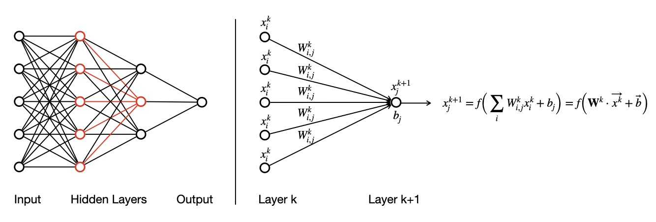
Neural networks are flexible computational models that can process inputs and produce outputs, with parameters that can be fit or estimated based on data. They represent a type of computational graph inspired by the action of neurons in the brain. The structure of these models reflects a directed network of artificial "neurons" or nodes, in which data are presented as inputs to a network, those inputs are fed through the neural network architecture — which includes one or more hidden layers — and which ultimately produces outputs. This general architecture is represented schematically in the left panel of the figure below. It is conventional to represent neural networks as flowing from left to right, with the input nodes on the far left and the output nodes on the far right. Within the illustration of an entire neural network, we highlight a subset of nodes and edges in red.
Just as the network as a whole includes a set of inputs and outputs, so does each individual node in the network, as illustrated in the right panel of the figure below. Each edge that connects two nodes carries with it an associated weight, indicating the strength of influence between the two nodes. In the network depicted below, for each node \(j\) in layer \(k+1\), a set of incoming inputs \(x^k_j\) are multiplied by the corresponding weights \(W^k_{i,j}\) along each edge, and those products are summed. Finally, a bias or offset \(b_j\) is added to the sum to define an aggregated, weighted input for that node. Computationally, this is accomplished as a matrix-vector multiplication involving the weight matrix \(\bar W^k\) and the node vector \(\vec x^k\), followed by the addition of the bias vector \(\vec b^k\). The value of that node \(x^{k+1}_j\) is computed by applying an activation function \(f\) to the aggregated input. That output \(x^{k+1}_j\) then serves as an input to downstream nodes in the network. The right panel of the figure below illustrates this action for one node in the network, but all other nodes in the network are updated simultaneously in an analogous manner, each with its own set of inputs and edge weights. Inputs are mapped through all the internal (hidden) layers of the network until an output is produced at the end.
The action of the network is parameterized by the edge weights \(\bar W\) and the biases \(\vec b\). Depending on the numerical values of those parameters, the outputs computed by the network, for a given set of inputs, can vary. The "learning" that is at the core of deep learning is the determination of suitable values for those numerical parameters that do a good job of producing a mapping (function) between the inputs and the outputs. One property that makes neural networks very powerful in this task is that they are universal functional approximators: with a sufficient number of nodes, a neural network can approximate any sufficiently smooth function that maps inputs to outputs.
Training, learning, and parameter estimation
A model is trained — that is, its parameters are estimated from data — by making iterative modifications to the parameter values in order to reduce the loss associated with the current set of parameter values. This is typical of many optimization algorithms in scientific computing, where one wishes to move "downhill" along the loss surface (see figure below). With neural networks, deciding how specifically to change the values of parameters in order to move most quickly downhill is aided by a process known as backpropagation. Leveraging the magic of calculus and a computational technique known as
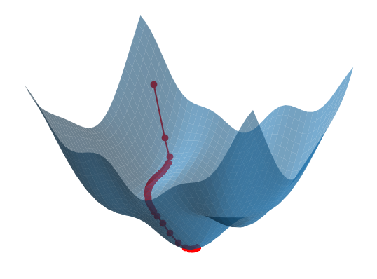
Image credit: I did a Google search asking something like "Produce some code using matplotlib to generate a 3D plot of a wavy surface, along with a path starting from a point on that surface and moving downhill by gradient descent." And the Google AI Overview produced some code that I used as a starting point to generate this figure. I wanted to tweak the specific function being used to represent the 3D surface, which also required my recomputing the gradient of that new function, since the gradient of the original function was hardwired into the code that Google produced. I also tweaked some of the details of the plotting.
Designing an appropriate network architecture for a given problem is itself an art and a science, the details of which are beyond the scope of this tutorial. For certain classes of problems, however, there are architectural elements that are regularly used, such as convolutional layers for image processing applications and transformer architectures for large language models. We discuss this in a bit more detail on the following page.
CVW material development is supported by NSF OAC awards 1854828, 2321040, 2323116 (UT Austin) and 2005506 (Indiana University)