DeepONet (Deep Operator Network) is the practical implementation of the Operator Universal Approximation Theorem.

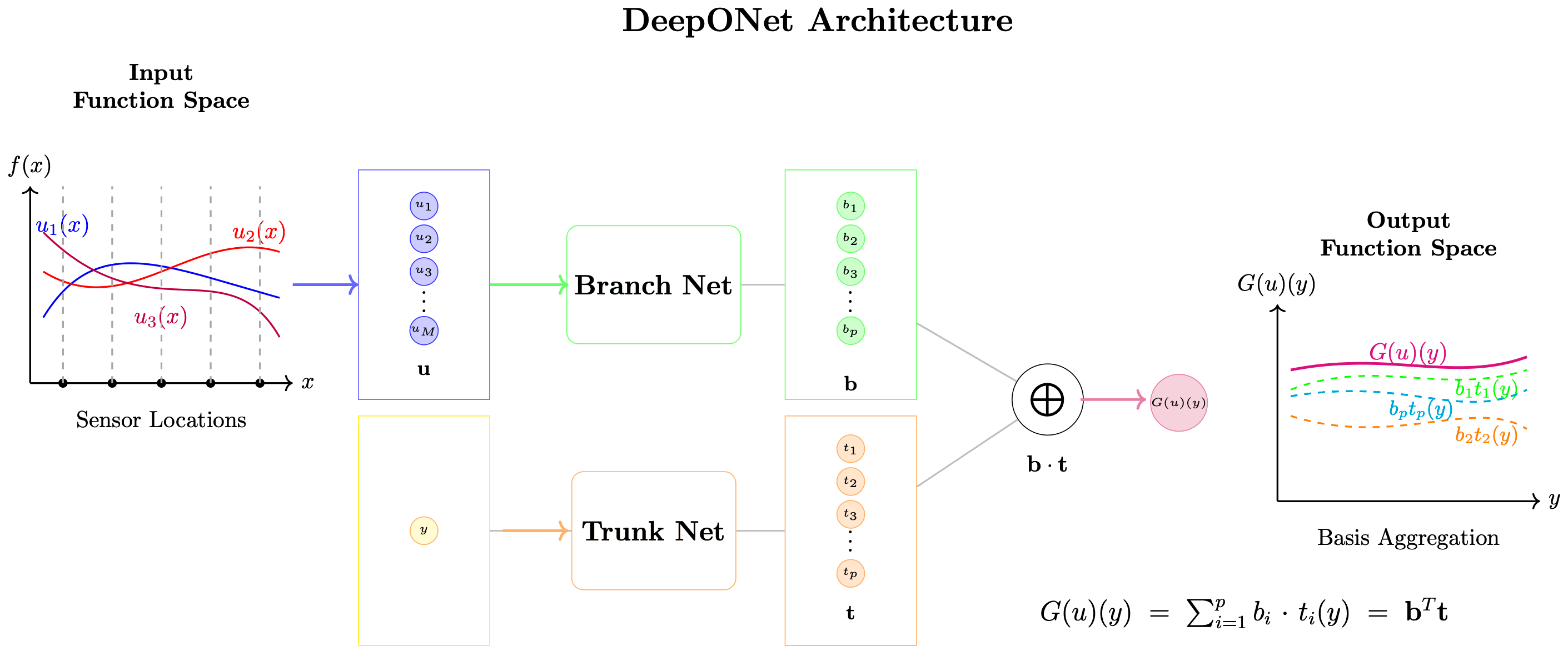
Core Architecture

where:

• Branch network: \( b_k(u) = \mathcal{B}_k([u(x_1), u(x_2), \ldots, u(x_m)]) \)
• Trunk network: \( t_k(y) = \mathcal{T}_k(y) \)
• \( p \): Number of basis functions (typically 50-200)
• \( b_0 \): Bias term

Training Data Structure

Input-output pairs: \( (u^{(i)}, y^{(j)}, \mathcal{G}(u^{(i)})(y^{(j)})) \)

• \( N \) input functions: \( \{u^{(i)}\}_{i=1}^N \)
• Each function sampled at \( m \) sensors: \( \{u^{(i)}(x_j)\}_{j=1}^m \)
• Corresponding outputs at query points: \( \{\mathcal{G}(u^{(i)})(y_k)\} \)

Loss Function

Key Advantages

1. Resolution independence: Train on one grid, evaluate on any grid
2. Fast evaluation: Once trained, instant prediction (no iterative solving)
3. Generalization: Works for new functions not seen during training
4. Physical consistency: Learns the underlying operator