The Programmable Filter is very similar to the Programmable Source, and that section should be studied before continuing with this section. Where the Programmable Source can only generate new data for the visualization pipeline, the Programmable Filter can also manipulate existing pipeline data from one or more inputs. Programmable Filters can generate new data arrays, modify existing ones, and even convert one type of data into a completely different type.

Much as with the Python Calculator, you must select all desired input nodes before instantiating a Programmable Filter. Each of these input nodes will then be joined to the set of identical Programmable Filter nodes that are created simulataneously. All input nodes must have the same geometric topology and dimensions, and the output of the Python Filter will contain the geometry from the first input node. For simplicity, in this section we will only be working with a single input node.

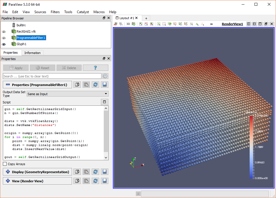
Let's explore the Programmable Filter by creating a script that adds a scalar data array to the existing rectilinear grid data in the pipeline. The array will be associated with the node's point data, and each value will hold the point's distance from one corner of the grid. A Glyph filter will allow the distances to be visualized using the default color map. We begin by adding the grid data, then the Programmable Filter and Glyph:

• Edit→Reset Session.
• File→Open and select the RectGrid2.vtk data set. Click "Apply".
• Filters→Data Analysis→Programmable Filter.
• "Output Data Set Type" must be set to "Same as Input" for this example.
• Copy the script below and paste it into the Script section, then click "Apply".
• With the ProgrammableFilter selected use Filters→Glyph to add a Glyph filter.
• Set Glyph Type to "Sphere".
• Set Scale Array to "No scale array".
• Set Scale Factor to 0.05.
• Set Glyph Mode to "All Points".
• Set Coloring to "distances".
• Click "Apply".

gin = self.GetRectilinearGridInput()
n = gin.GetNumberOfPoints()

dists = vtk.vtkFloatArray()
dists.SetName("distances")

origin = numpy.array(gin.GetPoint(0))
for i in range(0, n):
    point = numpy.array(gin.GetPoint(i))
    dist = numpy.linalg.norm(point - origin)
    dists.InsertNextValue(dist)

gout = self.GetRectilinearGridOutput()
gout.GetPointData().SetScalars(dists)

The first block of code in this script accesses the input grid geometry and uses it to determine how many points are in its collection. The second block of code asks the VTK library to allocate an empty floating point data array and assigns it the desired name, "distances".

The third block of code gets the first point of the input data and converts it to a NumPy array, a data type that is needed for a later calculation. It then iterates over all the points in the input data, getting each point's location as a NymPy array and using NumPy's linear algebra library to calculate its distance from the origin. Each point's distance value is then appended to the scalar data array.

In the final code block the output grid geometry is accessed and the newly created scalar data array is assigned to it. When we click "Apply", the script is executed and the new data array can be seen in the node's Information panel and is accessible to the Glpyh filter that follows.