Multi-Layer Perceptron (MLP)
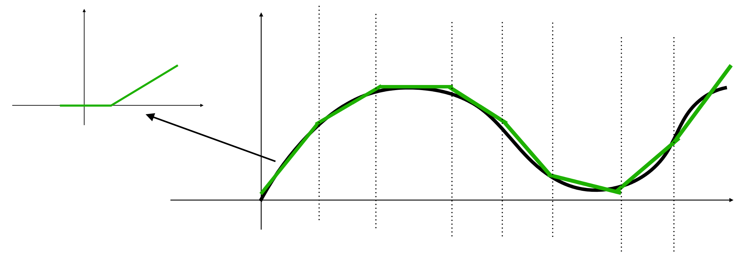
When MLP is applied to a linear regression problem, it can be considered as building a piecewise linear function to simulate the target curve.
Layers in MLP are called linear layers or fully connected layers. Neurons in each layer are fully connected to the neurons in the following layer. The Figure below shows an example of MLP for binary classification.
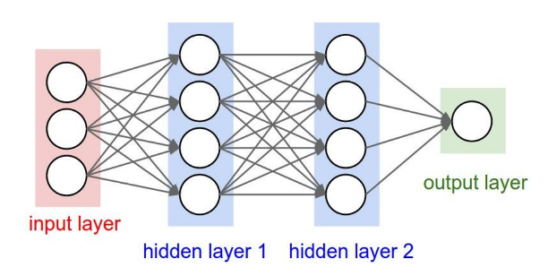
Image source: [1]
Here are some terminologies for a MLP:
Here is the formula for the MLP shown in the figure:
For binary classification (i.e. dataset has only two possible labels), we can define one class with label 1 and the other class with label -1, and then use the sign of \(𝑦∈\mathbb{R}\) as the classification result. For multiclass classification, we use one output per class that uses the softmax activation function.
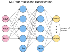
Image source: [2]
[1] Li. URL: https://cs231n.github.io/neural-networks-1/
[2] Opennn. URL: http://www.opennn.net/
CVW material development is supported by NSF OAC awards 1854828, 2321040, 2323116 (UT Austin) and 2005506 (Indiana University)