Gradient Descent

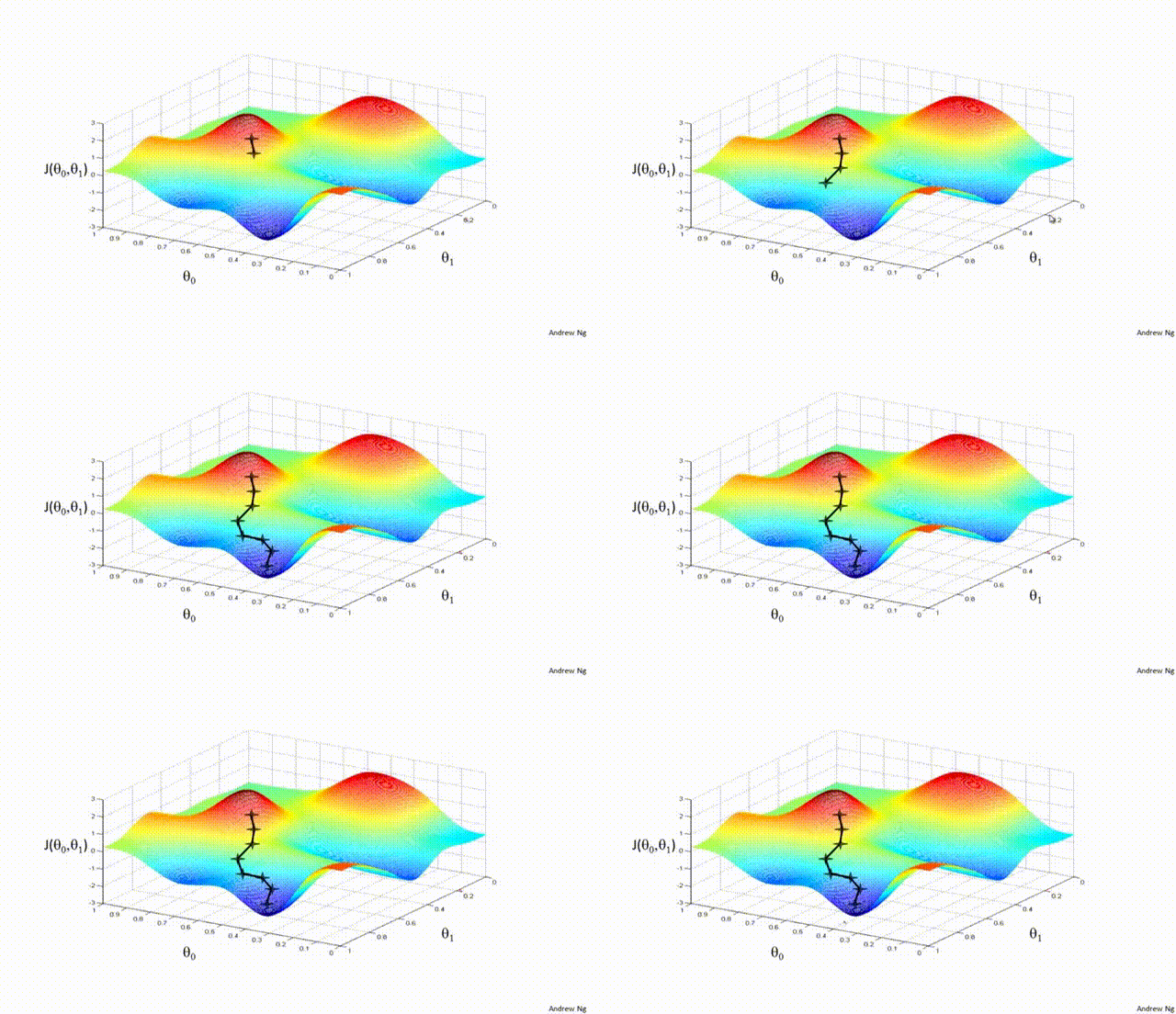
Gradient Descent is a first-order iterative optimization algorithm used to find the minimum of a differentiable function. In the context of training a neural network, we are trying to minimize the loss function.

1. Initialize Parameters:

   Choose an initial point (i.e., initial values for the weights and biases) in the parameter space, and set a learning rate that determines the step size in each iteration.

2. Compute the Gradient:

   Calculate the gradient of the loss function with respect to the parameters at the current point. The gradient is a vector that points in the direction of the steepest increase of the function. It is obtained by taking the partial derivatives of the loss function with respect to each parameter.

3. Update Parameters:

   Move in the opposite direction of the gradient by a distance proportional to the learning rate. This is done by subtracting the gradient times the learning rate from the current parameters:

   \[ \boldsymbol{w} = \boldsymbol{w} - \eta \nabla J(\boldsymbol{w}) \]

   Here, \(\boldsymbol{w}\) represents the parameters, \(\eta\) is the learning rate, and \(\nabla J (\boldsymbol{w})\) is the gradient of the loss function \(J\) with respect to \(\boldsymbol{w}\).

4. Repeat:

   Repeat steps 2 and 3 until the change in the loss function falls below a predefined threshold, or a maximum number of iterations is reached.

Algorithm:

1. Initialize weights randomly \(\sim \mathcal{N}(0, \sigma^2)\)
2. Loop until convergence
3. Compute gradient, \(\frac{\partial J(\boldsymbol{w})}{\partial \boldsymbol{w}}\)
4. Update weights, \(\boldsymbol{w} \leftarrow \boldsymbol{w} - \eta \frac{\partial J(\boldsymbol{w})}{\partial \boldsymbol{w}}\)
5. Return weights

Assuming a loss function is mean squared error (MSE). Let's compute the gradient of the loss with respect to the input weights.

The loss function is mean squared error:

Where \(y_i\) are the true target and \(\hat{y}_i\) are the predicted values.

To minimize this loss, we need to compute the gradients with respect to the weights \(\mathbf{w}\) and bias \(b\):

Using the chain rule, the gradient of the loss with respect to the weights is:

The term inside the sum is the gradient of the loss with respect to the output \(y_i\), which we called grad_output:

The derivative \(\frac{\partial y_i}{\partial \mathbf{w}}\) is just the input \(\mathbf{x}_i\) multiplied by the derivative of the activation. For simplicity, let's assume linear activation, so this is just \(\mathbf{x}_i\):

The gradient for the bias is simpler:

Finally, we update the weights and bias by gradient descent:

Where \(\eta\) is the learning rate.

Variants:

There are several variants of Gradient Descent that modify or enhance these basic steps, including:

• Stochastic Gradient Descent (SGD): Instead of using the entire dataset to compute the gradient, SGD uses a single random data point (or small batch) at each iteration. This adds noise to the gradient but often speeds up convergence and can escape local minima.
• Momentum: Momentum methods use a moving average of past gradients to dampen oscillations and accelerate convergence, especially in cases where the loss surface has steep valleys.
• Adaptive Learning Rate Methods: Techniques like Adagrad, RMSprop, and Adam adjust the learning rate individually for each parameter, often leading to faster convergence.

Limitations:

• It may converge to a local minimum instead of a global minimum if the loss surface is not convex.
• Convergence can be slow if the learning rate is not properly tuned.
• Sensitive to the scaling of features; poorly scaled data can cause the gradient descent to take a long time to converge or even diverge.

Effect of learning rate

The learning rate in gradient descent is a critical hyperparameter that can significantly influence the model's training dynamics. Let us now look at how the learning rate affects local minima, overshooting, and convergence:

1. Effect on Local Minima:
   • High Learning Rate: A large learning rate can help the model escape shallow local minima, leading to the discovery of deeper (potentially global) minima. However, it can also cause instability, making it hard to settle in a good solution.
   • Low Learning Rate: A small learning rate may cause the model to get stuck in local minima, especially in complex loss landscapes with many shallow valleys. The model can lack the 'energy' to escape these regions.
2. Effect on Overshooting:
   • High Learning Rate: If the learning rate is set too high, the updates may be so large that they overshoot the minimum and cause the algorithm to diverge, or oscillate back and forth across the valley without ever reaching the bottom. This oscillation can be detrimental to convergence.
   • Low Learning Rate: A very low learning rate will likely avoid overshooting but may lead to extremely slow convergence, as the updates to the parameters will be minimal. It might result in getting stuck in plateau regions where the gradient is small.
3. Effect on Convergence:
   • High Learning Rate: While it can speed up convergence initially, a too-large learning rate risks instability and divergence, as mentioned above. The model may never converge to a satisfactory solution.
   • Low Learning Rate: A small learning rate ensures more stable and reliable convergence but can significantly slow down the process. If set too low, it may also lead to premature convergence to a suboptimal solution.

Finding the Right Balance:

Choosing the right learning rate is often a trial-and-error process, sometimes guided by techniques like learning rate schedules or adaptive learning rate algorithms like Adam. These approaches attempt to balance the trade-offs by adjusting the learning rate throughout training, often starting with larger values to escape local minima and avoid plateaus, then reducing it to stabilize convergence.