Reverse mode AD (also called backpropagation) computes derivatives by propagating derivative information backward through the computational graph.

The Backward Pass Algorithm

1. Forward pass: Compute function values and store intermediate results
2. Seed the output: Set \(\bar{y} = 1\) (derivative of output w.r.t. itself)
3. Backward pass: Use the chain rule to propagate derivatives backward

Computing All Partial Derivatives in One Pass

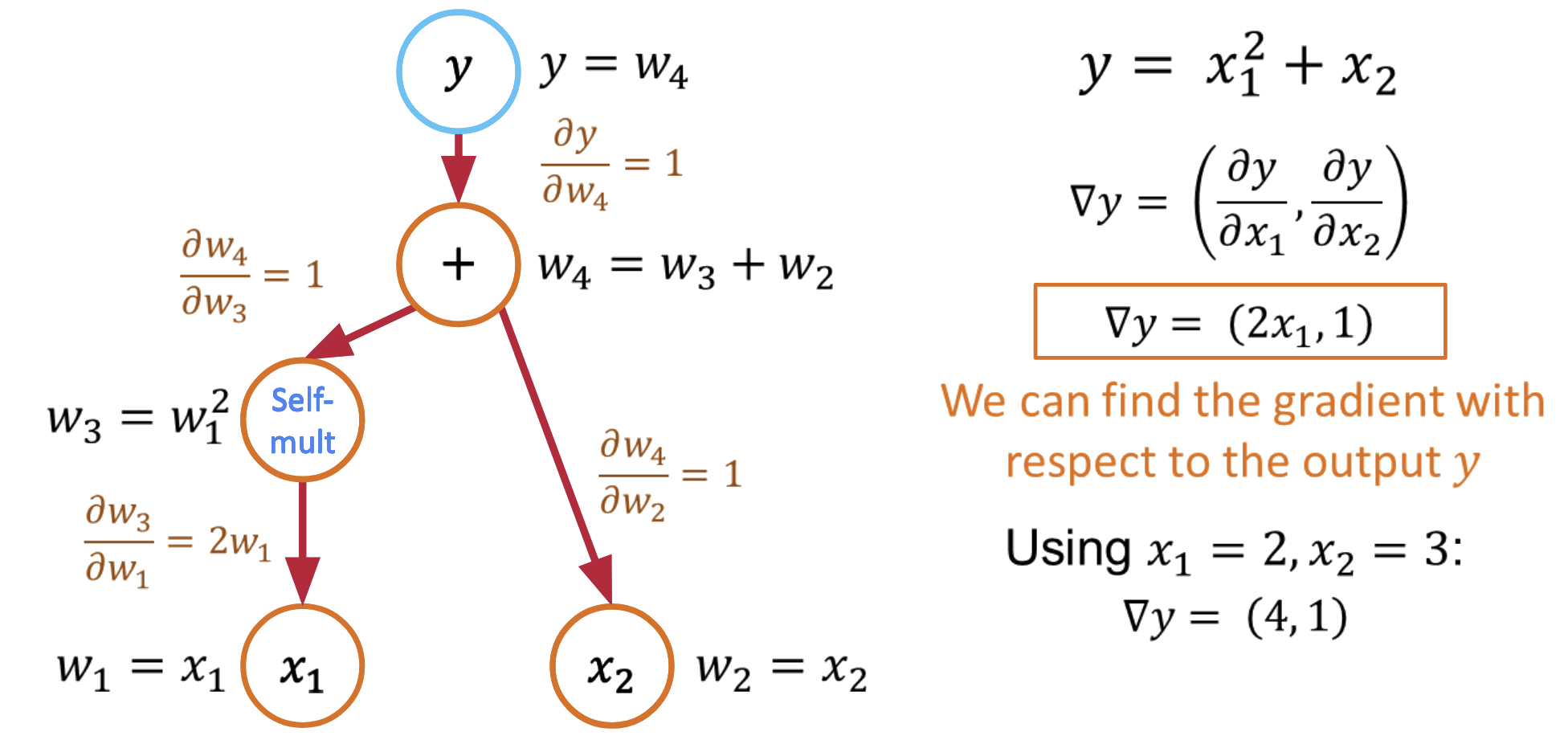
The beauty of reverse mode is that it computes all partial derivatives in a single backward pass:

1. Forward pass: \(y = x_1^2 + x_2\) (store intermediate values)
2. Backward pass with \(\bar{y} = 1\):
   • \(\frac{\partial y}{\partial x_1} = \frac{\partial y}{\partial v_1} \cdot \frac{\partial v_1}{\partial x_1} = 1 \cdot 2x_1 = 2x_1\)
   • \(\frac{\partial y}{\partial x_2} = \frac{\partial y}{\partial x_2} = 1\)

AD: The Mathematical Foundation

Automatic differentiation works because of a fundamental theorem:

Chain Rule: For composite functions \(f(g(x))\):

By systematically applying the chain rule to each operation in a computational graph, AD can compute exact derivatives for arbitrarily complex functions.

Automatic Differentiation in Practice: PyTorch

Let's see how automatic differentiation works in PyTorch:

A More Complex Example: Neural Network

When to Use Forward vs Reverse Mode

The choice depends on the structure of your problem:

• Forward Mode: Efficient when few inputs, many outputs (e.g., \(f: \mathbb{R}^n \to \mathbb{R}^m\) with \(n \ll m\))
• Reverse Mode: Efficient when many inputs, few outputs (e.g., \(f: \mathbb{R}^n \to \mathbb{R}^m\) with \(n \gg m\))

In machine learning, we typically have millions of parameters (inputs) and a single loss function (output), making reverse mode the natural choice.