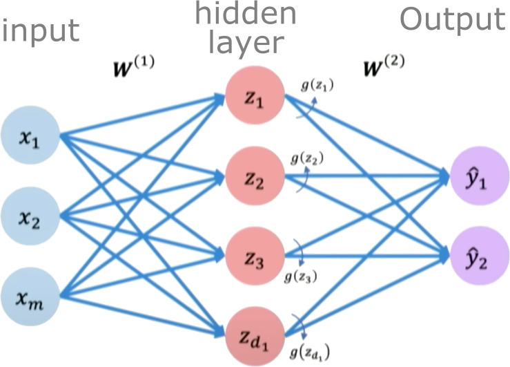
A single perceptron is limited in the complexity of functions it can represent. To increase capacity, we combine multiple perceptrons into a layer. A single-layer feedforward neural network (also known as a shallow Multi-Layer Perceptron or MLP) consists of an input layer, one hidden layer of neurons, and an output layer.

For our 1D input \(x\), a single-layer network with \(N_h\) hidden neurons works as follows:

1. Input Layer: Receives the input \(x\).
2. Hidden Layer: Each of the \(N_h\) neurons in this layer performs a linear transformation on the input \(x\) and applies a non-linear activation function \(g\). The output of this layer is a vector \(\boldsymbol{h}\) of size \(N_h\).
   • Pre-activation vector \(\boldsymbol{z}^{(1)}\) (size \(N_h\)): \(\boldsymbol{z}^{(1)} = W^{(1)}\boldsymbol{x} + \boldsymbol{b}^{(1)}\)
     (Here, \(W^{(1)}\) is a \(N_h \times 1\) weight matrix, \(\boldsymbol{x}\) is treated as a \(1 \times 1\) vector, and \(\boldsymbol{b}^{(1)}\) is a \(N_h \times 1\) bias vector).
   • Activation vector \(\boldsymbol{h}\) (size \(N_h\)): \(\boldsymbol{h} = g(\boldsymbol{z}^{(1)})\) (where \(g\) is applied element-wise).
3. Output Layer: This layer takes the vector \(\boldsymbol{h}\) from the hidden layer and performs another linear transformation to produce the final scalar output \(\hat{y}\). For regression, the output layer typically has a linear activation (or no activation function explicitly applied after the linear transformation).
   • Pre-activation scalar \(z^{(2)}\): \(z^{(2)} = W^{(2)}\boldsymbol{h} + b^{(2)}\)
     (Here, \(W^{(2)}\) is a \(1 \times N_h\) weight matrix, and \(b^{(2)}\) is a scalar bias).
   • Final output \(\hat{y}\): \(\hat{y} = z^{(2)}\)