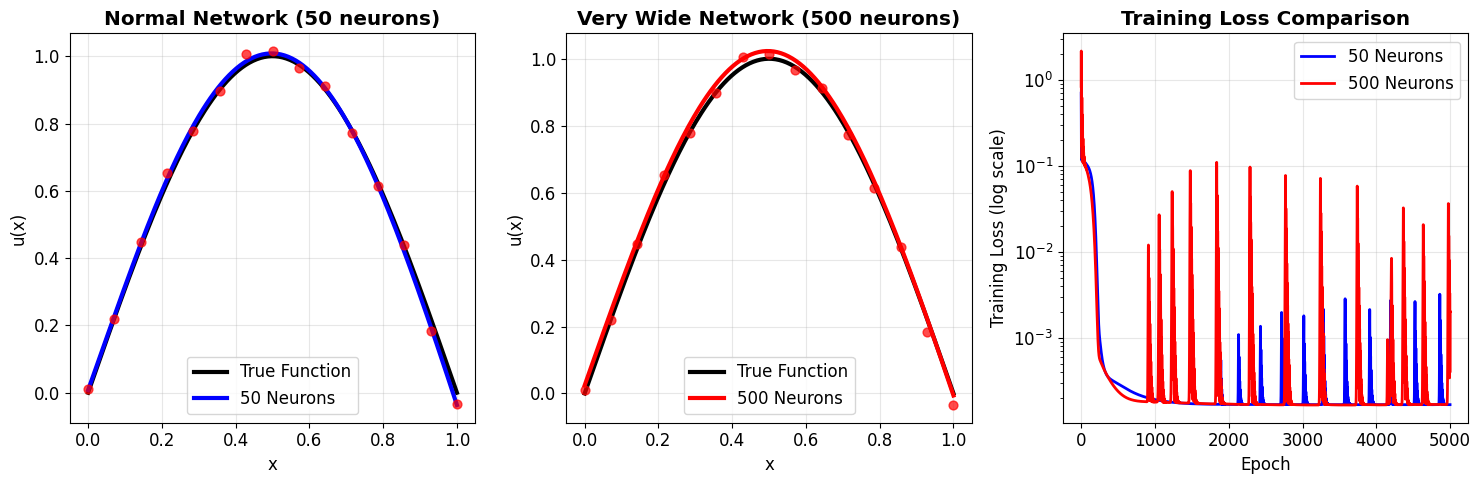
The visualizations from our experiment in The Key Experiment: Width vs Approximation Quality show a clear trend: as we increased the number of neurons in the hidden layer (the network's width), the network's ability to approximate the \(\sin(\pi x)\) function significantly improved, and the final training loss decreased.

This experimental result experimentally validates the statement of the Universal Approximation Theorem – a single hidden layer with non-linearity does have the capacity to approximate continuous functions, and increasing the number of neurons provides more of this capacity, allowing it to better fit the target function.

However, the theorem guarantees existence, not practicality. Our experiment also hints at practical considerations:

• Number of Neurons Needed: While 50 neurons did a good job for \(\sin(\pi x)\), approximating more complex functions might require a very large number of neurons in a single layer. This can be computationally expensive and require a lot of data.
• Training Difficulty: The theorem doesn't guarantee that gradient descent will successfully find the optimal parameters. Training can be challenging, especially for very wide networks or complex functions.
• Remaining Errors: Even with 50 neurons, there's still some error. For more complex functions or higher accuracy requirements, a single layer might struggle or need excessive width.

Practical Considerations: Overfitting and Hyperparameters

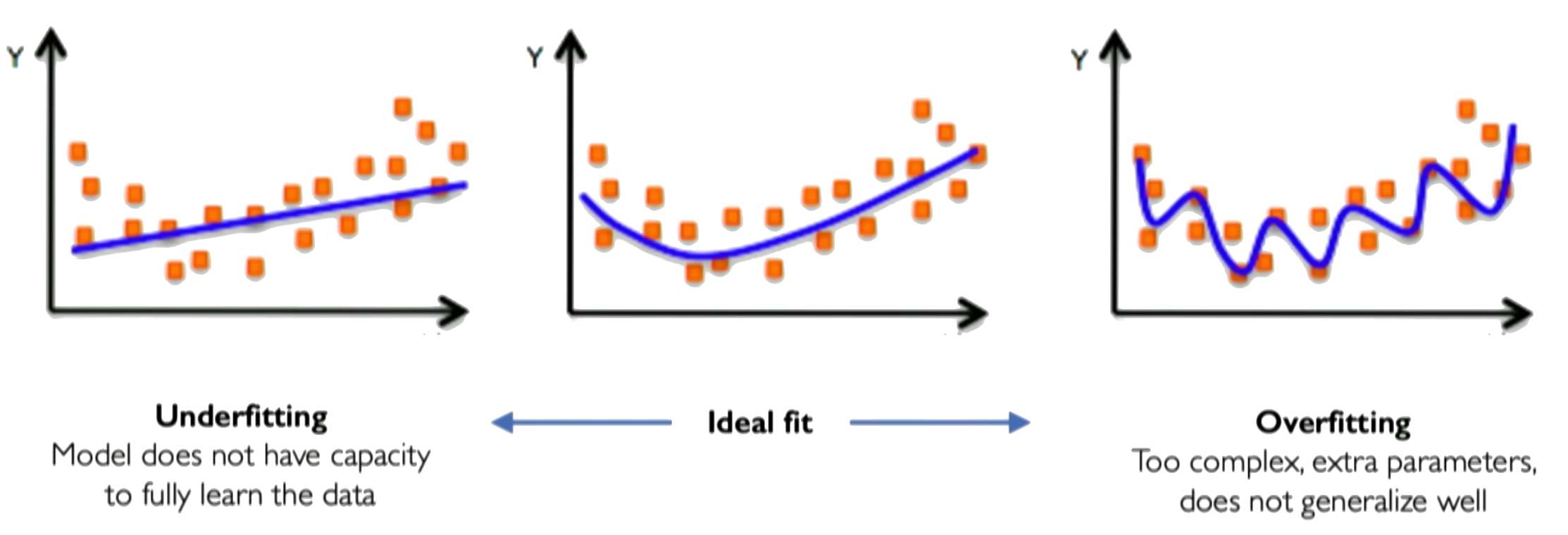
As network capacity increases (e.g., by adding more neurons), there's a risk of overfitting. This occurs when the model learns the training data (including noise) too well, capturing spurious patterns that don't generalize to unseen data, leading to poor performance outside the training set.

Overfitting can be detected by monitoring performance on a separate validation set during training. If the validation loss starts increasing while the training loss continues to decrease, it's a sign of overfitting.

Strategies to mitigate overfitting include using more training data, regularization techniques, early stopping (stopping training when validation performance degrades), or reducing model complexity.

Problem: High-capacity networks can memorize training data instead of learning the true function

Detection: Monitor validation loss - if it increases while training loss decreases, you're overfitting

Solutions:

• More training data
• Regularization (L1/L2, dropout)
• Early stopping
• Simpler architectures

Hyperparameter Choices

Hyperparameters are settings chosen before training that significantly influence the learning process and the final model. Key hyperparameters we've encountered include:

• Learning Rate (\(\eta\)): Controls the step size in gradient descent. Too high can cause divergence; too low can lead to slow convergence or getting stuck in local minima.
• Number of Epochs: How many times the training data is passed through the network. Too few may result in underfitting; too many can cause overfitting.
• Hidden Layer Size (\(N_h\)): The number of neurons in the hidden layer. Impacts model capacity. Too small can underfit; too large can overfit.
• Choice of Activation Function: Impacts the network's ability to model specific shapes and the training dynamics (e.g., Tanh/Sigmoid for smooth functions but potential vanishing gradients, ReLU for efficiency but 'dead neuron' issue). The best choice can be problem-dependent.

Finding the right balance of hyperparameters is crucial for successful training and generalization.

How to detect overfitting with validation dataset

In practice, the learning algorithm does not actually find the best function, but merely one thatsignificantly reduces the training error. These additional limitations, such as theimperfection of the optimization algorithm, mean that the learning algorithm’seffective capacitymay be less than the representational capacity of the modelfamily.

Our modern ideas about improving the generalization of machine learningmodels are refinements of thought dating back to philosophers at least as early as Ptolemy. Many early scholars invoke a principle of parsimony that is now mostwidely known as Occam’s razor (c. 1287–1347). This principle states that amongcompeting hypotheses that explain known observations equally well, we shouldchoose the “simplest” one. This idea was formalized and made more precise in the twentieth century by the founders of statistical learning theory.

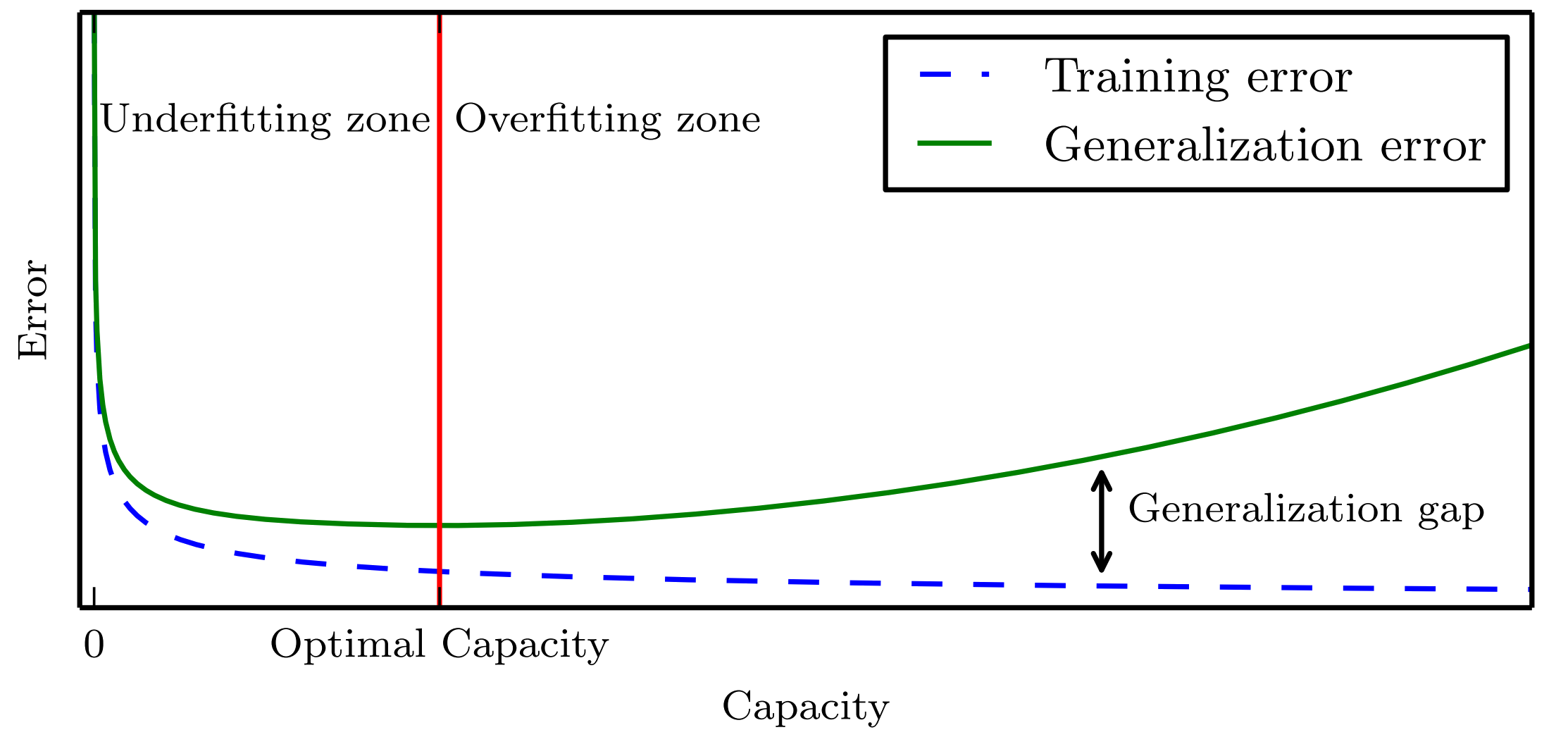
We must remember that while simpler functions are more likely to generalize (to have a small gap between training and test error), we must still choose a sufficiently complex hypothesis to achieve low training error. Typically, training error decreases until it asymptotes to the minimum possible error value as model capacity increases (assuming the error measure has a minimum value). Typically generalization error has a U-shaped curve as a function of model capacity.

At the left end of the graph, training error and generalization error are both high. This is the underfitting region. As we increase capacity, training error decreases, but the gap between training and generalization error increases. Eventually, the size of this gap outweighs the decrease in training error, and we enter the overfitting region, where capacity is too large, above the optimal capacity.

The story so far: Single-layer networks can approximate any function (Universal Approximation) but may need impractically many neurons. The question: Can depth be more efficient than width?