The most common way to enforce boundary conditions in a PINN is the "soft" or "weak" method. The core idea is to treat the boundary conditions just like the PDE itself: as a component of the total loss function that we want to minimize.

How it works:

1. We define a boundary loss term, \( \mathcal{L}_{BC} \), which measures the mean squared error between the network's predictions at the boundary points and the true boundary values.
2. This boundary loss is added to the PDE residual loss, \( \mathcal{L}_{PDE} \), often with a weighting factor \( \lambda_{BC} \).
3. The total loss is: \( \mathcal{L}_{\text{total}} = \mathcal{L}_{PDE} + \lambda_{BC} \mathcal{L}_{BC} \).

By minimizing \( \mathcal{L}_{\text{total}} \), the optimizer is encouraged to find a solution that approximately satisfies the boundary conditions. Satisfaction is not guaranteed by the network's structure but is instead a goal of the optimization. The weight \( \lambda_{BC} \) is a hyperparameter that balances how strictly the boundary conditions are enforced relative to the PDE.

PINN Definition and Loss Functions

First, we define our neural network and the two loss components.

Training the Soft-Constraint PINN

Now, we set up the training loop. We sample points inside the domain (collocation points) to enforce the PDE and points on the boundary to enforce the BCs. We choose a large weight lambda_bc to strongly encourage the network to satisfy the boundary conditions.

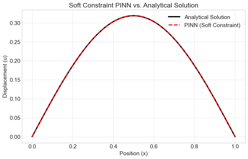
As we can see, the soft constraint approach produces a very accurate solution. However, the predicted values at the boundaries are not exactly zero, but very small numbers. This is the nature of soft enforcement—it gets close, but not perfect, depending on the loss weight and training.