Stage 1: Understanding the Forward Problem
Stage 1: Understanding the Forward Problem
Before tackling the inverse problem, let's understand the forward problem and generate our "experimental" data.
Analytical Solution
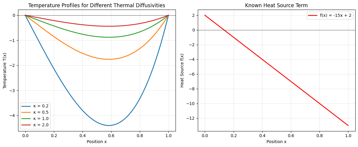
For our specific case with \( f(x) = -15x + 2 \) and homogeneous boundary conditions, the exact solution is:
\[ T(x) = \frac{15x^3 - 2x^2 - 13x}{6\kappa} \]
Key insight:
Notice how \( T(x) \) depends on \( \kappa \). Different values of \( \kappa \) give different temperature profiles!
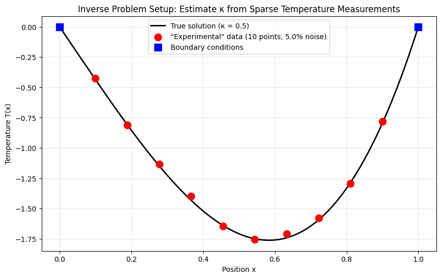
Creating "Experimental" Data
In a real experiment, we would measure temperature at a few locations. Let's simulate this with sparse, noisy measurements.
©
|
Cornell University
|
Center for Advanced Computing
|
Copyright Statement
|
Access Statement
CVW material development is supported by NSF OAC awards 1854828, 2321040, 2323116 (UT Austin) and 2005506 (Indiana University)
CVW material development is supported by NSF OAC awards 1854828, 2321040, 2323116 (UT Austin) and 2005506 (Indiana University)