Before we dive into implementation, we need to understand why neural networks can solve differential equations. The answer lies in the Universal Approximation Theorem and its extension to Sobolev spaces.

Classical Universal Approximation Theorem

As we learned in the MLP module, the classical UAT tells us that feedforward networks can approximate continuous functions:

Theorem (Cybenko, 1989): Let \( \sigma \) be a continuous, non-constant, and bounded activation function. Then finite sums of the form:

are dense in \( C(K) \) for any compact set \( K \subset \mathbb{R}^d \).

Translation: Given enough neurons, neural networks can approximate any continuous function arbitrarily well.

Extension to Sobolev Spaces: The Key for PDEs

This is where Sobolev spaces become essential.

Definition (Sobolev Space \( H^k(\Omega) \)): The space of functions whose weak derivatives up to order \( k \) are square-integrable:

where \( D^\alpha u \) denotes the weak derivative of multi-index \( \alpha \) with \( |\alpha| = \alpha_1 + \alpha_2 + \cdots + \alpha_d \).

Extended Universal Approximation Theorem: Neural networks with sufficiently smooth activation functions can approximate functions in Sobolev spaces \( H^k(\Omega) \).

Mathematical Statement: Let \( \sigma \in C^k(\mathbb{R}) \) (i.e., \( \sigma \) is \( k \) times continuously differentiable). Then for any \( u \in H^k(\Omega) \) and \( \epsilon > 0 \), there exists a neural network \( \hat{u}_\theta \) such that:

where the Sobolev norm is:

Why This Matters for PINNs

Critical Connection: When we solve a differential equation of order \( k \), we need:

1. Function approximation: \( \hat{u}_\theta(x) \approx u(x) \)
2. Derivative approximation: \( \frac{\partial^j \hat{u}_\theta}{\partial x^j} \approx \frac{\partial^j u}{\partial x^j} \) for \( j = 1, 2, \ldots, k \)

The extended UAT guarantees this is possible provided:

• Activation function smoothness: \( \sigma \in C^k \) (at least \( k \) times differentiable)
• Sufficient network capacity: Enough neurons and layers

For our oscillator ODE: \( m\frac{d^2u}{dt^2} + c\frac{du}{dt} + ku = 0 \)

• We need \( k = 2 \) (second-order equation)
• Activation function must be \( C^2 \) (twice differentiable)
• \( \tanh \), \( \sin \), Swish ✓ | ReLU ✗

The Magic: Automatic differentiation + UAT in Sobolev spaces = neural networks that can learn solutions to differential equations!

Training the Standard Neural Network

What we expect: The network should learn to pass through the data points.

What we hope: It will interpolate smoothly between points.

What actually happens: Let's find out!

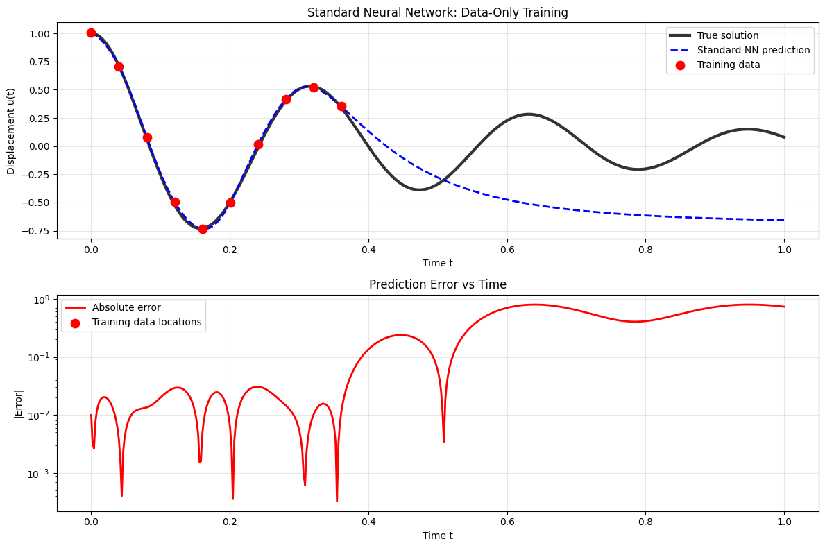
The Failure of the Data-Only Approach

Critical Question: How well does it predict the full solution?

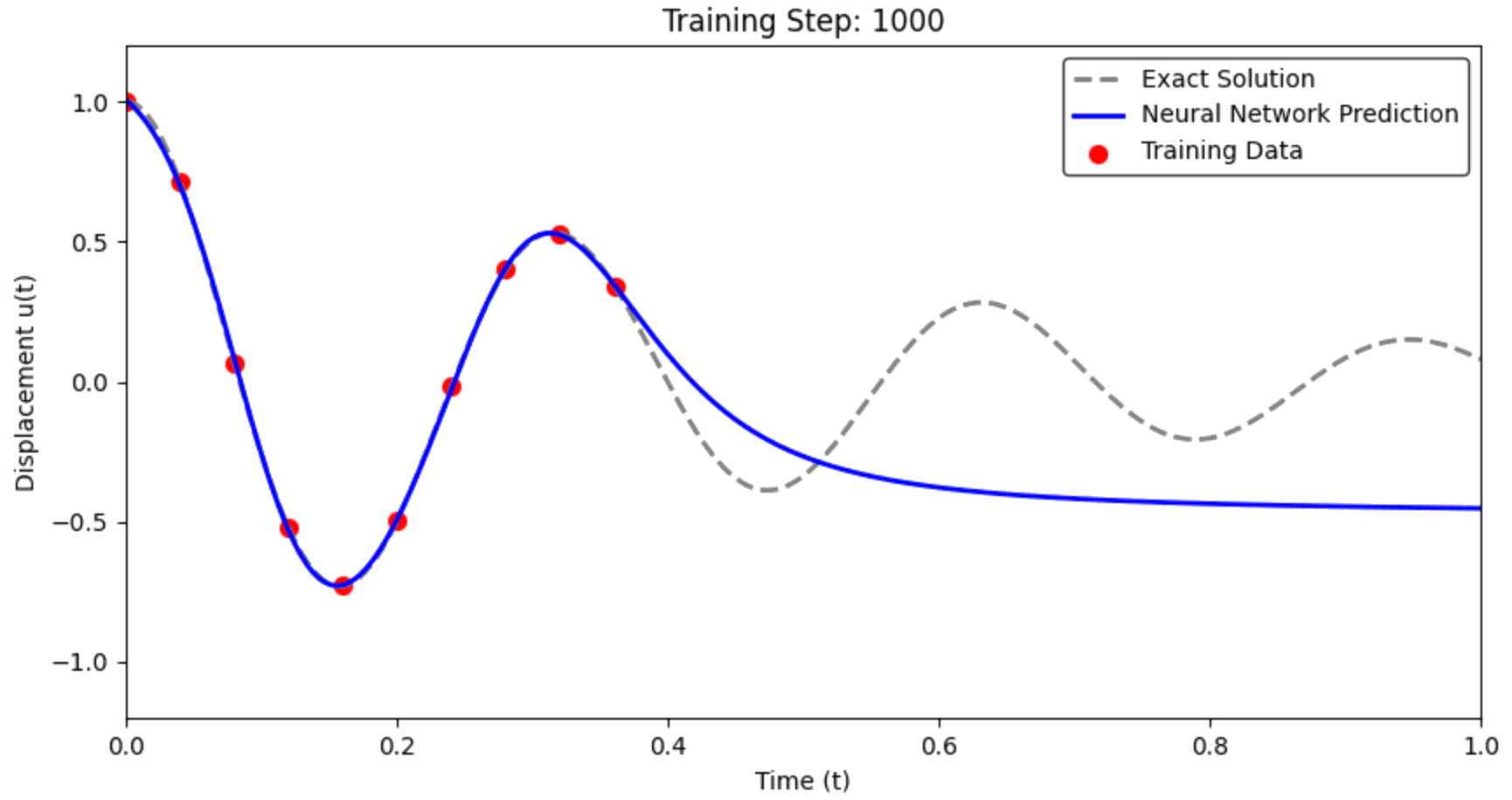
What we observe: The network fits the training points but fails catastrophically between them.