An alternative to penalty terms is to enforce the boundary conditions by construction. This is known as the "hard" or "strong" method.

How it works: We redefine the network's output to create a "trial solution" \( \tilde{u}(x) \) that is mathematically guaranteed to satisfy the Dirichlet boundary conditions, regardless of the neural network's raw output.

For our problem with BCs \( u(0)=0 \) and \( u(1)=0 \), a suitable trial solution is:

where \( \text{NN}(x; \theta) \) is the output of a standard neural network and \( D(x) \) is a function that is zero at the boundaries. A simple and effective choice is:

Our new model's output is \( \tilde{u}(x) = x(1-x)\text{NN}(x; \theta) \).

• At \( x=0 \), \( \tilde{u}(0) = 0 \cdot (1-0) \cdot \text{NN}(0) = 0 \).
• At \( x=1 \), \( \tilde{u}(1) = 1 \cdot (1-1) \cdot \text{NN}(1) = 0 \).

The BCs are now satisfied exactly. The training process simplifies significantly, as the loss function now only contains the PDE residual term. We no longer need a boundary loss or a weighting hyperparameter.

PINN Definition for Hard Constraints

We create a new model that wraps our original PINN and applies the hard constraint transformation.

Training the Hard-Constraint PINN

The training loop is now simpler, with only the PDE loss to minimize.

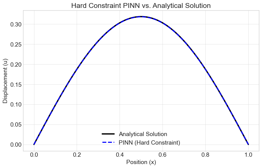
With the hard constraint, the predicted values at the boundaries are exactly zero, as expected from the design.